本文对openMVG 2.1中的sift相关源码进行了解析，算法原理部分请见上一篇文章万字长文详解SIFT特征提取，本文代码中涉及的一些细节问题可以当作上一篇文章的补充。

调用例程

openMVG的项目源代码中有sift的调用例程，见：
openMVG-2.1\src\openMVG_Samples\features_siftPutativeMatches\siftmatch.cpp

其中核心调用sift的代码：

using namespace openMVG::features;
std::unique_ptr<Image_describer> image_describer(new SIFT_Anatomy_Image_describer);  //核心类初始化，具体分析见下文
std::map<IndexT, std::unique_ptr<features::Regions>> regions_perImage; //用于储存特征
image_describer->Describe(imageL, regions_perImage[0]); //主要执行函数
image_describer->Describe(imageR, regions_perImage[1]);

SIFT_Anatomy_Image_describer类

算法的核心类为 SIFT_Anatomy_Image_describer，位于SIFT_Anatomy_Image_Describer.hpp中

核心参数设置

其参数有一个struct传入，在初始化时会有一个默认的参数值初始化，如下：

    Params(
      int first_octave = 0, //如果设置为-1，则第一个octave中使用的是扩大一倍的图像，也就是upscale一次
      int num_octaves = 6, //最大的octave数量
      int num_scales = 3,     // 每层octave输出的尺度数量
      float edge_threshold = 10.0f, // 去除边缘时用到的阈值
      float peak_threshold = 0.04f,  // 去除对比度小的点时用到的阈值
      bool root_sift = true  // 是否使用改进的sift描述符

first_octave，在openMVG中，默认的首层octave图像是源图像大小，可以通过这个参数设置为扩大一倍的大小。这里upscale主要是为了能够检测到更加细节的特征，此外，如果原图的分辨率本身较低，upscale一下也有助于检测到小尺度特征。
另，在opencv中，是直接默认首层upscale的。

num_octaves，设置的最大octave数量，此外，在后面的代码中还会根据图片尺寸算一个octave数量，来保证最后一层的分辨率不要太小（不小于32X32），在HierarchicalGaussianScaleSpace类中我们详细介绍。

num_scales每个octave的输出scale数量，这个数量加3，就是每个octave所需要的高斯层数量。

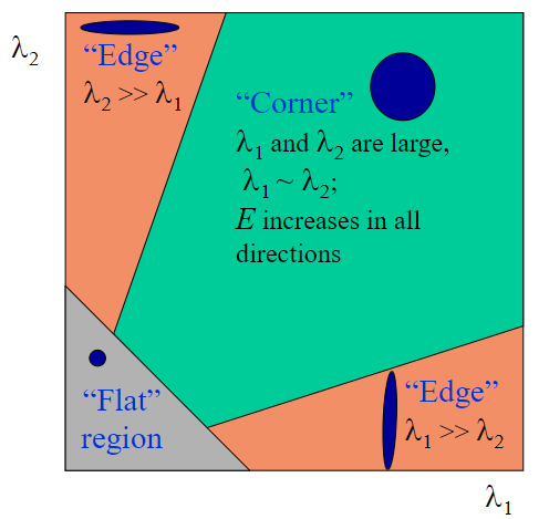
edge_threshold这里判定是否为边缘点的方法和之前原理篇讲的略有不同，但原理基本一致，都是得到局部Hessian矩阵后，判断特征值的大小情况。
在之前的判定中，我们计算出Hessian矩阵M后，采用这个公式计算其R响应：

\[R = \text{Det}(M) – \alpha \text{Tr}(M)^2=\lambda_{1}\lambda_{2}-\alpha(\lambda_{1}+\lambda_{2})^2 \]

其中α是一个经验值 0.04 到 0.06。

但在openMVG中，我们假设 $$λ_1 = γλ_2$$
其中γ > 1，该值越大，表示两者之间的比值越大，越有可能是边缘。

我们采用trace平方和determinant的比值来判定：

\[\frac{\mathrm{Tr}(\boldsymbol{M})^2}{\mathrm{Det}(\boldsymbol{M})}=\frac{(\lambda_1 + \lambda_2)^2}{\lambda_1\lambda_2}=\frac{(\gamma\lambda_2+\lambda_2)^2}{\gamma\lambda_2^2}=\frac{(\gamma + 1)^2}{\gamma} \]

这里如果得到的值越大，表示γ的值越大，也就表示越有可能是边缘点。edge_threshold就是这里设置的γ，SIFT原作者给出一个经验值10，在openMVG中也是用的这个经验值。

peak_threshold这个用来去掉对比度小的点，计算方法我们在SIFT_KeypointExtractor类中详述。

root_sift改进的sift描述符，详见Sift_DescriptorExtractor类。

算法流程核心 Describe_SIFT_Anatomy

包含整体的特征提取算法流程。核心流程函数！

std::unique_ptr<Regions_type> Describe_SIFT_Anatomy(
  const image::Image<unsigned char>& image,    
  const image::Image<unsigned char>* mask = nullptr  
)
//image：传入图像
//mask：掩码图像，用于过滤关键点。非零值表示感兴趣区域。通常传一个空即可
{
  auto regions = std::unique_ptr<Regions_type>(new Regions_type);

  if (image.size() == 0)
    return regions;

  // Convert to float in range [0;1]
  //将输入图像转换为浮点数类型，并将像素值归一化到 [0, 1] 范围
  const image::Image<float> If(image.GetMat().cast<float>()/255.0f);

  // compute sift keypoints
  // 计算 SIFT 关键点
  {
    const int supplementary_images = 3;
    // 高斯层数和输出尺度之间的数量差3，详见sift原理文章。
    // => in order to ensure each gaussian slice is used in the process 3 extra images are required:
    // +1 for dog computation
    // +2 for 3d discrete extrema definition

    //生成高斯尺度空间，详见后文具体的类分析
    HierarchicalGaussianScaleSpace octave_gen(
      params_.num_octaves_,
      params_.num_scales_,
      (params_.first_octave_ == -1) // 这里判定首个octave是否要upscale，如果要upscale，相关尺度要进行调整
      ? GaussianScaleSpaceParams(1.6f/2.0f, 1.0f/2.0f, 0.5f, supplementary_images)
      : GaussianScaleSpaceParams(1.6f, 1.0f, 0.5f, supplementary_images));
    octave_gen.SetImage( If );  //设置输入图像，详见下文相关类分析

    std::vector<sift::Keypoint> keypoints; // 存储所有检测到的关键点
    keypoints.reserve(5000);  // 预分配空间，提高性能
    Octave octave; // 存储当前octave的信息，以后每次迭代都是修改这个里面的信息
    while ( octave_gen.NextOctave( octave ) )  // 遍历octave
    {
      std::vector<sift::Keypoint> keys;
      // Find Keypoints 创建一个 SIFT 关键点检测器
      sift::SIFT_KeypointExtractor keypointDetector(
        params_.peak_threshold_ / octave_gen.NbSlice(),  
        params_.edge_threshold_);
    //参数1：这里就是原理篇中讲的对比度阈值计算方法，其中peak_threshold_为经验值
    //参数2：边缘阈值，详见上文
      keypointDetector(octave, keys); // 检测关键点，详细过程见下文
      // 创建一个 SIFT 描述符提取器
      sift::Sift_DescriptorExtractor descriptorExtractor;
      descriptorExtractor(octave, keys); // 计算当前octave中关键点的方向和描述符

      // Concatenate the found keypoints
      std::move(keys.begin(), keys.end(), std::back_inserter(keypoints));
    }
    for (const auto & k : keypoints)
    {
      // Feature masking 特征掩码处理
      if (mask)
      {
        const image::Image<unsigned char> & maskIma = *mask;
        if (maskIma(k.y, k.x) == 0) // 如果关键点位于掩码的非感兴趣区域，则跳过该关键点
          continue;
      }
      // Create the SIFT region 创建 SIFT 区域
      {
        // 将关键点的描述符转换为无符号字符类型，并添加到 Regions 对象中
          regions->Descriptors().emplace_back(k.descr.cast<unsigned char>());
          // 将关键点的坐标、尺度和方向添加到 Regions 对象中
          regions->Features().emplace_back(k.x, k.y, k.sigma, k.theta);
      }
    }
  }
  return regions;
};

在构建高斯金字塔时，往GaussianScaleSpaceParams(1.6f/2.0f, 1.0f/2.0f, 0.5f, supplementary_images)中传了一个0.5，我们默认输入图像已经进行了一次高斯卷积操作，其σ为这个0.5，那么第一层的图像就是从这个0.5卷积后的图像基础上，再进行一次卷积得到的。如果第一层所需的σ为1.6，则再次卷积所需的高斯σ为：

\[\sigma_{extra} = \sqrt{1.6^2-0.5^2} \]

而不是直接对图像做σ为1.6的卷积。

HierarchicalGaussianScaleSpace类

构建高斯金字塔的核心类

设置初始图象 SetImage

设置初始图像，主要是判断是否要upscale，以及计算octave的数量。

  virtual void SetImage(const image::Image<float> & img)
  {
    const double sigma_extra =
      sqrt(Square(m_params.sigma_min) - Square(m_params.sigma_in)) / m_params.delta_min; // 计算额外的高斯模糊标准差，用于在图像上应用额外的高斯滤波，见上文分析
    if (m_params.delta_min == 1.0f) // 如果最小采样距离为 1.0f，直接对输入图像应用高斯滤波
    {
      image::ImageGaussianFilter(img, sigma_extra, m_cur_base_octave_image);
    }
    else  // 如果最小采样距离为 0.5f，需要对图像进行上采样
    {
      if (m_params.delta_min == 0.5f)
      {
        image::Image<float> tmp;
        ImageUpsample(img, tmp); //上采样
        image::ImageGaussianFilter(tmp, sigma_extra, m_cur_base_octave_image);
      }
      else
      {
        OPENMVG_LOG_ERROR
          << "Upsampling or downsampling with delta equal to: "
          << m_params.delta_min << " is not yet implemented";
      }
    }
    //-- Limit the size of the last octave to be at least 32x32 pixels
    // 保证最后一个octave至少为 32x32 像素，这个要和传入的最大octave数量做个对比，取小的那个作为octave数量的确定值
    const int nbOctaveMax = std::ceil(std::log2( std::min(m_cur_base_octave_image.Width(), m_cur_base_octave_image.Height())/32));
    m_nb_octave = std::min(m_nb_octave, nbOctaveMax);
  }

octave的最大数量，是根据图片分辨率得到的，取分辨率长宽的较小值除以32，再以2为底求log，向上取整得到。这个值和传入参数的设定值取较小值作为最终的octave数量。

\[\text{nbOctaveMax} = \left\lceil \log_2 \left( \frac{\min(\text{ImageWidth}, \text{ImageHeight})}{32} \right) \right\rceil\]

迭代 NextOctave

构建下一层octave，是构建高斯金字塔的关键函数。

  virtual bool NextOctave(Octave & octave)
  {
    if (m_cur_octave_id >= m_nb_octave)
    {
      return false;  // 如果达到最大数量，返回 false 表示没有更多的octave可供计算
    }
    else
    {
      octave.octave_level = m_cur_octave_id;
      if (m_cur_octave_id == 0) // 如果是第一个octave
      {
        octave.delta = m_params.delta_min; //设置采样率为最小采样率
      }
      else
      {
        octave.delta *= 2.0f; // 对于后续的octave，采样率翻倍（相当于图像缩小）
      }

      // init the "blur"/sigma scale spaces values
      octave.slices.resize(m_nb_slice + m_params.supplementary_levels);
      octave.sigmas.resize(m_nb_slice + m_params.supplementary_levels);
      for (int s = 0; s < m_nb_slice  + m_params.supplementary_levels; ++s)
      {
        octave.sigmas[s] =
          octave.delta / m_params.delta_min * m_params.sigma_min * pow(2.0,(float)s/(float)m_nb_slice);   //这里计算octave内每一层所需的sigma，其中k = 2^{1/s}，详见原理篇文章
      }

      // Build the octave iteratively
      octave.slices[0] = m_cur_base_octave_image;
      for (int s = 1; s < octave.sigmas.size(); ++s)
      {
        // Iterative blurring the previous image
        const image::Image<float> & im_prev = octave.slices[s-1];
        image::Image<float> & im_next = octave.slices[s];
        const double sig_prev = octave.sigmas[s-1];
        const double sig_next = octave.sigmas[s];
        const double sigma_extra = sqrt(Square(sig_next) - Square(sig_prev)) / octave.delta;  // 下一层的sigma是由当前层再进行一次卷积得到的，这个额外的卷积核计算方法遵循勾股定理

        image::ImageGaussianFilter(im_prev, sigma_extra, im_next); //高斯模糊生成该层图像，每一层都是由上一层进行卷积的到，而非由原始图像卷积得到
      }
 
      // Prepare for next octave computation -> Decimation
      ++m_cur_octave_id;
      if (m_cur_octave_id < m_nb_octave)
      {
        // Decimate => sigma * 2 for the next iteration
        const int index = (m_params.supplementary_levels == 0) ? 1 : m_params.supplementary_levels;
        // 对选定的切片进行下采样，作为下一个octave的基础图像
        ImageDecimate(octave.slices[octave.sigmas.size()-index], m_cur_base_octave_image);
      }
      return true;
    }
  }

const int index = (m_params.supplementary_levels == 0) ? 1 : m_params.supplementary_levels; 这里我们用第一个octave举例，如果supplementary_levels为3，则index = 3，那么下采样的层就是第6-3=3层，也就是sigma为\(2σ_{initial}\)的层，把这层作为第二个octave的基础图象。也就是说本来第二个octave的基础图象应该是\(2σ_{initial}\)对原图做卷积，这在第一个octave中已经计算过了，可以直接拿到第二个octave中去用。

SIFT_KeypointExtractor类

特征点提取类。在每一个octave迭代时，包含两个关键步骤，极值提取、极值修正。

默认参数

    float peak_threshold,     // 对比度阈值，详见上文
    float edge_threshold,     // 边缘去除阈值，详见上文
    int nb_refinement_step = 5 // 极值修正是一个迭代过程，这里限制了最大迭代次数

核心流程

  // 重载函数调用运算符，计算给定高斯octave的差分高斯（DoG），并在 DoG 空间中查找离散极值点
  //对这些关键点的位置进行细化，以得到更精确的关键点位置。
  void operator()( const Octave & octave , std::vector<Keypoint> & keypoints )
  {
    if (!ComputeDogs(octave)) // 差分高斯（DoG），就是两个图像相减，不再赘述
      return;
    Find_3d_discrete_extrema(keypoints, 0.8f);   //找到离散极值点，这里的0.8是对对比度阈值的一次缩放，可以初步筛出更多的极值点；默认值为1，对原阈值不做修改
    Keypoints_refine_position(keypoints);        //对极值点进行修正
  }

极值提取 Find_3d_discrete_extrema

在 DoG 空间中查找 3D 离散极值点

//遍历DoG金字塔的每个切片，在每个切片的每个像素点上，查找其3D空间3X3X3的局部空间最大值或最小值。
//只有当像素值的绝对值超过设定的峰值阈值时，才会进一步检查其是否为局部极值。
//如果是局部极值，则将其作为候选关键点保存。
void Find_3d_discrete_extrema
(
  std::vector<Keypoint> & keypoints,
  float percent = 1.0f
) const
{
  const int ns = m_Dogs.slices.size();
  const float delta = m_Dogs.delta;
  const int h = m_Dogs.slices[0].Height();
  const int w = m_Dogs.slices[0].Width();

  // Loop through the slices of the image stack (one octave)
  for (int s = 1; s < ns-1; ++s) // 遍历slice
  {
    for (int id_row = 1; id_row < h-1; ++id_row ) //遍历行
    {
      for (int id_col = 1; id_col < w-1; ++id_col ) // 遍历列
      {
        const float pix_val = m_Dogs.slices[s](id_row, id_col); //经过一通遍历得到像素值
        if (std::abs(pix_val) > m_peak_threshold * percent) // 对比度高的点才进行后续判定
        if (is_local_min_max(m_Dogs.slices, s, id_row, id_col)) // 与周围26个邻居比大小
        {
          // if 3d discrete extrema, save a candidate keypoint
          //发现极值点！加入
          Keypoint key;
          key.i = id_col;
          key.j = id_row;
          key.s = s;
          key.o = m_Dogs.octave_level;
          key.x = delta * id_col;
          key.y = delta * id_row;
          key.sigma = m_Dogs.sigmas[s];
          key.val = pix_val;
          keypoints.push_back(std::move(key));
        }
      }
    }
  }
  keypoints.shrink_to_fit();
}

极值修正 Keypoints_refine_position

细化关键点的位置（空间位置和尺度），丢弃无法细化的关键点

//遍历输入的关键点列表，对每个关键点进行位置细化。
//通过二次函数插值来优化关键点的位置，直到满足收敛条件或达到最大迭代次数。
//对细化后的关键点进行峰值阈值、边缘响应和边界检查，只有通过所有检查的关键点才会被保留。
void Keypoints_refine_position
(
  std::vector<Keypoint> & keypoints
) const
{
  std::vector<Keypoint> kps;
  kps.reserve(keypoints.size());

  const float ofstMax = 0.6f; // 细化参数的最大偏移量

  // Ratio between two consecutive scales in the slice
  // 这个就是k
  const float sigma_ratio = m_Dogs.sigmas[1] / m_Dogs.sigmas[0];
  // 边缘响应阈值, 计算原理详见上文
  const float edge_thres = Square(m_edge_threshold + 1) / m_edge_threshold;

  const Octave & octave = m_Dogs;
  const int w = octave.slices[0].Width();
  const int h = octave.slices[0].Height();
  const float delta  = octave.delta;

  for (const auto & key : keypoints) // 遍历keypoints
  {
    float val = key.val;

    int ic = key.i; // current discrete value of x coordinate - at each interpolation
    int jc = key.j; // current discrete value of y coordinate - at each interpolation
    int sc = key.s; // current discrete value of s coordinate - at each interpolation

    float ofstX = 0.0f;
    float ofstY = 0.0f;
    float ofstS = 0.0f;

    bool isConv = false;
    // While position cannot be refined and the number of refinement is not too much
    // 迭代细化极值点
    for ( int nIntrp = 0; !isConv && nIntrp < m_nb_refinement_step; ++nIntrp)
    {
      // Extrema interpolation via a quadratic function
      //   only if the detection is not too close to the border (so the discrete 3D Hessian is well defined)
      if ( 0 < ic &&  ic < (w-1) && 0 < jc && jc < (h-1) )
      {
        // 通过taylor展开得到极值点附近的二次项近似，求取极值点偏移，求解过程实际是解一个导数为0的方程，详见算法原理篇
        if (Inverse_3D_Taylor_second_order_expansion(octave, ic, jc, sc, &ofstX, &ofstY, &ofstS, &val, ofstMax))
          isConv = true;
      }
      else
      {
        isConv = false;
      }
      if (!isConv)
      {
        // let's explore the neighborhood in
        // space...
        if (ofstX > +ofstMax && (ic+1) < (w-1) ) {++ic;}
        if (ofstX < -ofstMax && (ic-1) >  0    ) {--ic;}
        if (ofstY > +ofstMax && (jc+1) < (h-1) ) {++jc;}
        if (ofstY < -ofstMax && (jc-1) >  0    ) {--jc;}
        // ... and scale.
        /*
        if (ofstS > +ofstMax && (sc+1) < (ns-1)) {++sc;}
        if (ofstS < -ofstMax && (sc-1) >    0  ) {--sc;}
        */
      }
    }

    if (isConv)
    {
      // Peak threshold check
      if ( std::abs(val) > m_peak_threshold )  // 对比度高的点保留
      {
        Keypoint kp = key;
        kp.x = (ic + ofstX) * delta;
        kp.y = (jc + ofstY) * delta;
        kp.i = ic;
        kp.j = jc;
        kp.s = sc;
        kp.sigma = octave.sigmas[sc] * pow(sigma_ratio, ofstS); // logarithmic scale
        kp.val = val;
        // Edge check 高斯差分对边缘的响应也很高，要把这些边缘点去除掉
        if (Compute_edge_response(kp) >=0 && std::abs(kp.edgeResp) <= edge_thres)
        {
          // Border check 边界点去除
          if (Border_Check(kp, w, h))
          {
            kps.push_back(std::move(kp));
          }
        }
      }
    }
  }
  keypoints = std::move(kps);
  keypoints.shrink_to_fit();
}

边缘响应计算 Compute_edge_response

  //计算关键点所在位置的 2D 海森矩阵（Hessian matrix），
  //根据前文所述方法计算边缘响应值。
  //边缘响应值用于判断关键点是否位于边缘上，避免在边缘上检测到过多的关键点。
  float Compute_edge_response
  (
    Keypoint & key
  ) const
  {
    const int s = key.s;
    const int i = key.i; // i = id_row
    const int j = key.j; // j = id_col
    const Octave & octave = m_Dogs;
    const image::Image<float> & im = octave.slices[s];
    //  计算2D 海森矩阵（Hessian matrix）
    const float hXX = im(j,i-1) + im(j,i+1) - 2.f * im(j,i);
    const float hYY = im(j+1,i) + im(j-1,i) - 2.f * im(j,i);
    const float hXY = ((im(j+1,i+1) - im(j-1,i+1)) - ((im(j+1,i-1) - im(j-1,i-1))))/4.f;
    // Harris and Stephen Edge response
    key.edgeResp = Square(hXX + hYY)/(hXX*hYY - hXY*hXY);
    return key.edgeResp;
  }

计算前文所述的公式：

\[\frac{\mathrm{Tr}(\boldsymbol{M})^2}{\mathrm{Det}(\boldsymbol{M})}=\frac{(\lambda_1 + \lambda_2)^2}{\lambda_1\lambda_2}=\frac{(\gamma\lambda_2+\lambda_2)^2}{\gamma\lambda_2^2}=\frac{(\gamma + 1)^2}{\gamma} \]

Sift_DescriptorExtractor类

SIFT描述符生成类，该类主要用作方向计算和描述符生成。

默认参数

    // Orientation computation parameters
    const int nb_orientation_histogram_bin = 36, //用于计算关键点方向的方向直方图的bin数量，默认为36，也就是每10度为一个bin
    const float orientation_scale = 1.5f,//设置方向计算时局部半径宽度缩放
    const int nb_smoothing_step = 6,   //在计算关键点方向之前，对方向直方图的平滑步骤数
    const float percentage_keep = 0.8f,//高于该百分比的最高方向直方图值将用于计算新的方向
    
    // Descriptor computation parameters
    const bool b_root_sift = true,  //是否计算根SIFT归一化直方图
    const float descriptor_scale = 6.0f,  //描述符框计算的尺度，设置描述符补丁的宽度
    const int nb_split2d = 4,  //应用于描述符直方图的x和y方向的分割数
    const int nb_split_angle = 8,  //应用于描述符直方图的z方向的分割数
    const float clip_value = 0.2f  //在计算最终描述符之前，高于此阈值的值将被截断

核心流程

void operator()
(
  const Octave & octave,
  std::vector<Keypoint> & keypoints
)
{
  Compute_Gradients(octave);          //梯度计算
  Keypoints_orientations(keypoints);  //关键点方向计算
  Keypoints_description(keypoints);   //关键点描述符生成
}

算梯度 Compute_Gradients

//计算高斯octave中每个切片x和y方向的梯度，并将结果分别存储在 `m_xgradient` 和 `m_ygradient` 中。
//由于第一个和最后一个切片仅用于非极大值抑制，因此只计算中间切片的梯度。
  void Compute_Gradients(const Octave & octave)
  {
    const int nSca = octave.slices.size();
    m_xgradient.slices.resize(nSca);
    m_ygradient.slices.resize(nSca);
    m_xgradient.delta = octave.delta;
    m_ygradient.delta = octave.delta;
    m_xgradient.octave_level = octave.octave_level;
    m_ygradient.octave_level = octave.octave_level;
    for (int s = 1; s < nSca-1; ++s)
    {
      // 中心差分法计算梯度，卷积核为Vec3 kernel( -1.0, 0.0, 1.0 );
      image::ImageXDerivative( octave.slices[s], m_xgradient.slices[s]);
      image::ImageYDerivative( octave.slices[s], m_ygradient.slices[s]);
    }
  }

方向计算 Keypoints_orientations

//遍历关键点，为每个关键点计算方向直方图，
//然后从直方图中提取主方向，并将具有主方向的关键点保存到新列表中。
//最后，将新列表赋值给原始关键点列表。
  void Keypoints_orientations
  (
    std::vector<Keypoint> & keypoints
  ) const
  {
    std::vector<Keypoint> kps;
    kps.reserve(keypoints.size());
#ifdef OPENMVG_USE_OPENMP
#pragma omp parallel for schedule(dynamic)
#endif
    for (int i_key = 0; i_key < keypoints.size(); ++i_key)
    {
      const Keypoint & key = keypoints[i_key];

      openMVG::Vecf orientation_histogram; // 存储当前关键点的方向直方图
      // 计算当前关键点的方向直方图，详见下文分析
      Keypoint_orientation_histogram(key, orientation_histogram);

      //存储当前关键点的主方向
      std::vector<float> principal_orientations(m_nb_orientation_histogram_bin);
      // 从方向直方图中提取主方向，并返回主方向的数量，详见下文分析
      const int n_prOri = Extract_principal_orientations(orientation_histogram, principal_orientations);

      // Updating keypoints and save it in the new list
#ifdef OPENMVG_USE_OPENMP
      #pragma omp critical
#endif      
      // 遍历所有主方向
      for (int n = 0; n < n_prOri; ++n)
      {
        Keypoint kp = key;
        kp.theta = principal_orientations[n];        
        // 将带有方向信息的关键点添加到新列表中
        kps.push_back(std::move(kp));
      }
    }
    keypoints = std::move(kps);
    keypoints.shrink_to_fit();
  }

这里对于直方图的分析，与原理篇内容也略有不同，在实际代码中，若一个关键点存在多个主方向，针对每个主方向都会生成一个新的关键点，一个像素位置可能存在多个不同方向的关键点。在SIFT算法中，每个关键点的方向是依据其周围局部区域的梯度方向直方图来确定的。要是局部区域内的梯度方向分布较为复杂，就可能出现多个局部最大值，进而得到多个主方向。

这种处理方式能够提升特征的鲁棒性。因为不同方向的关键点能够捕捉到图像在不同方向上的特征信息，有助于在图像旋转或者视角变化的情况下仍能准确匹配。

在OpenCV中，除最大的主方向之外，其他主方向称为辅方向，原理一致。

方向直方图计算 Keypoint_orientation_histogram

计算以给定关键点为中心的局部区域内的梯度方向直方图。
梯度方向和幅值用于构建直方图，其中幅值经过高斯加权以减少远离关键点的像素的影响。

void Keypoint_orientation_histogram
  (
    const Keypoint & key,
    openMVG::Vecf & hist) const
  {

    hist.resize(m_nb_orientation_histogram_bin);
    hist.fill(0.0f); 

    // conversion to the octave's coordinates (sampling)
    const float delta  = m_xgradient.delta;
    const float x = key.x / delta;
    const float y = key.y / delta;
    const float sigma = key.sigma / delta;
  
    const int w = m_xgradient.slices[1].Width(); // 1 since 0 is empty
    const int h = m_xgradient.slices[1].Height();  
    
    // 获取当前尺度下的x和y方向的梯度图像
    const image::Image<float> & xgradient = m_xgradient.slices[key.s];
    const image::Image<float> & ygradient = m_ygradient.slices[key.s];  

    // 确定贡献像素所在的局部区域 [siMin;siMax] X [sjMin;sjMax]
    // 计算局部区域的半径
    const float R = 3 * m_orientation_scale * sigma;
    const int siMin = std::max(0, (int)(x - R + 0.5));
    const int sjMin = std::max(0, (int)(y - R + 0.5));
    const int siMax = std::min((int)(x + R + 0.5), w-1);
    const int sjMax = std::min((int)(y + R + 0.5), h-1);

    // 遍历局部区域内的每个像素
    for (int si = siMin; si <= siMax; ++si)
    {
      for (int sj = sjMin; sj <= sjMax; ++sj)
      {
        // 计算当前像素的梯度方向
        const float dx = xgradient(sj, si);
        const float dy = ygradient(sj, si);
        const float ori = modulus(atan2(dy, dx), 2*M_PI);  

        // 计算当前像素的梯度幅值，并应用高斯加权以减少远离关键点的像素的影响
        const float sX = (si - x) / sigma;
        const float sY = (sj - y) / sigma;
        const float r2 = Square(sX) + Square(sY); // 距离中心点距离，距离越远影响越小
        const float M = hypot(dx, dy) * exp(-r2/(2*Square(m_orientation_scale)));  //hypot(dx, dy) 计算的是当前像素的梯度幅值

        // 确定当前梯度方向在直方图中的bin索引
        const int gamma = ori_to_bin(ori, m_nb_orientation_histogram_bin);  

        // 将当前像素的梯度幅值贡献到对应的直方图bin中
        hist[gamma] += M;
      }
    }
  }

提取主方向 Extract_principal_orientations

从梯度方向直方图中提取主方向，局部最大值如果超过阈值（以最大值的百分比表示），则被视为次要主方向

int Extract_principal_orientations
  (
    openMVG::Vecf & orientation_histogram,
    std::vector<float> & principal_orientations
  ) const
  {
    // number of principal orientations (the return value).
    int o = 0;  

    // Smooth histogram : iterated box filters
    smooth_circular_histogram(m_nb_smoothing_step, orientation_histogram);  

    // What is the value of the global maximum
    const float max_value = orientation_histogram.maxCoeff();

    // 在直方图中搜索局部极值
    const int nbins = orientation_histogram.rows();

    for (int i = 0; i < nbins; ++i){

      const int i_prev = (i-1+nbins)%nbins;
      const int i_next = (i+1)%nbins;
      
      // 检查当前bin是否为局部最大值且超过阈值
      if ( (orientation_histogram[i] > m_percentage_keep * max_value)
        && (orientation_histogram[i]>orientation_histogram[i_prev])
        && (orientation_histogram[i]>orientation_histogram[i_next]))
      {
        // 对每个局部最大值的位置进行二次插值
        const float offset = interpolate_peak(orientation_histogram[i_prev], orientation_histogram[i], orientation_histogram[i_next]);
        // 将主方向（以[0, 2π]表示）添加到向量中
        principal_orientations[o] = bin_to_ori((float)i + offset, nbins);
        ++o;
      }
    }

    // return the number of principal orientations
    return o;
  }

描述符生成 Keypoints_description

//遍历输入的关键点列表，为每个关键点计算SIFT描述符，
//对描述符进行阈值处理，然后根据配置选择是否应用根SIFT归一化，
//最后对描述符进行量化，使其值范围在 [0; 255] 之间。
  void Keypoints_description
  (
    std::vector<Keypoint> & keypoints
  ) const
  {
    // 计算描述符的维度, 通常在x、y方向上各分为4份，每份计算8个角度，一共4X4X8=128 维向量
    const int n_descr = Square(m_nb_split2d) * m_nb_split_angle;
#ifdef OPENMVG_USE_OPENMP
#pragma omp parallel for schedule(dynamic)
#endif
    // 遍历所有关键点
    for (int i_key = 0; i_key < keypoints.size(); ++i_key)
    {
      Keypoint & key = keypoints[i_key];
      // Compute the SIFT descriptor
      key.descr.resize(n_descr);
      // 调用 Extract_sift_feature_vector 函数计算当前关键点的SIFT描述符，见下文详述
      Extract_sift_feature_vector(key, key.descr);

      // 计算描述符的L2范数，并添加一个极小值以避免除零错误
      float norm = key.descr.lpNorm<2>() + std::numeric_limits<float>::epsilon();
      // 对描述符的每个元素进行阈值处理，确保其不超过阈值 m_clip_value * norm
      for (int i = 0; i < key.descr.rows(); ++i){
        key.descr[i] = std::min(key.descr[i], m_clip_value * norm);
      }
      // 量化描述符
      if (m_b_root_sift)
      {        
        // 应用根SIFT归一化
        // 计算描述符的L1范数，并添加一个极小值以避免除零错误
        // scaling(rootsift) = sqrt( sift / sum(sift) );
        norm = key.descr.lpNorm<1>() + std::numeric_limits<float>::epsilon();
        // 对描述符进行根SIFT归一化，并乘以 512 进行量化
        key.descr = 512.f * (key.descr / norm).array().sqrt();
      }
      else
      {
        // 应用普通的L2归一化
        // 计算描述符的L2范数，并添加一个极小值以避免除零错误
        // scaling(normalized descriptor)
        norm = key.descr.lpNorm<2>() + std::numeric_limits<float>::epsilon();
        // 对描述符进行根SIFT归一化，并乘以 512 进行量化
        key.descr = 512.f * (key.descr / norm).array();
      }
    }
  }

Extract_sift_feature_vector

本节内容参考Opencv2.4.9源码分析——SIFT

每个特征点都包含坐标位置、尺度和方向。描述特征点是在该特征点所在的高斯尺度图像上进行的。在该图像上，以特征点为中心，将其附近邻域划分为4X4的子区域（SIFT原文）。每个子区域为一个正方形，边长为3σ。实际编程时特征邻域范围的边长设置为3σ(4+1)。

我们需要计算邻域范围内所有像素点的梯度幅值和幅角。幅值需要根据其对特征点中心的大小进行加权处理。

为保证旋转不变性，我们需要将特征区域旋转θ（特征点方向）。由于要保证旋转后区域包括整个正方形，旋转半径应设置为正方形对角线长的一半：

\[r=\frac{3 \sigma(4+1) \sqrt{2}}{2} \]

采样点旋转后的新坐标为:

\[\left[\begin{array}{l}x \\ y\end{array}\right]=\left[\begin{array}{rr}cos \theta & -sin \theta \\ sin \theta & cos \theta\end{array}\right]\left[\begin{array}{l}x \\ y\end{array}\right] \]

\[x, y \in[-r, r] \]

我们把邻域范围划分为16个子区域，每个区域内根据幅角大小放入不同的幅角bin中，每45度作为一个bin，一共8个bin。这样，我们就建立起了一个三维的直方图：

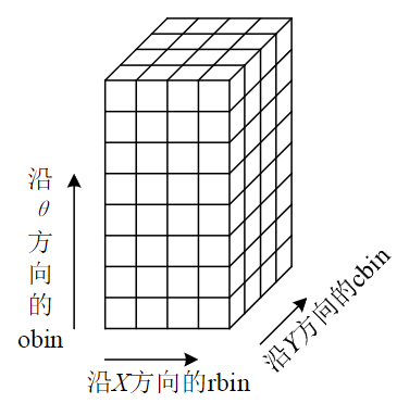
我们最终就是以这个直方图中一共128个bin中的值构建128维向量，作为我们的sift描述符。但在此之前，我们还需要做一些归一化处理。

首先，我们显然希望每个直方图中的小立方体的中心能够代表所有落入该小立方体的像素，然而每个像素落入直方图中的位置都不会在正中心位置，我们需要根据其相对正方体中心的位置进行加权处理。
然而，计算它们相对于中心点的加权过于繁琐，实际操作中我们是计算它们相对于正方体8个顶点的贡献大小

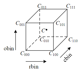
如图，点C(r, c, θ)对8个顶点的贡献分别为：

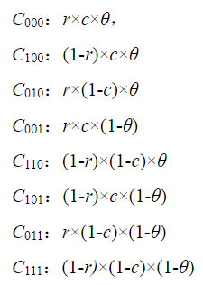
最终计算出该点特征矢量

\[P=\{p_{1}, p_{2}, …, p_{128}\} \]

再次进行归一化处理:

\[q_{i}=\frac{p_{i}}{\sqrt{\sum_{j=1}^{128} p_{j}}}, i=1,2, …, 128 \]

由于照相机饱和以及三维物体表面的不同数量不同角度的光照变化所引起的非线性光照变化，它能够影响到一些梯度的相对幅值，但不太会影响梯度幅角。为了消除这部分的影响，我们还需要设一个t=0.2 的阈值，也就是默认参数中的clip_value = 0.2f，以此保留 qi 中小于0.2 的元素，而把 大于0.2 的元素用0.2 替代。最后再进行一次归一化处理｡

来源链接：https://www.cnblogs.com/wangle1006/p/18791957